Timeseries analyis with Pandas pd.Grouper

Timeseries Analysis with Pandas - pd.Grouper

I have been doing time series analysis for some time in python. The pd.Grouper class used in unison with the groupy calls are extremely powerful and flexible. Understanding the framework of how to use it is easy, and once those hurdles are defined it is straight forward to use effectively.

I began to look into alternatives to excel (my companies standard), when I started to max out the limitations of excel:

  • limit the number of entries
  • calculation spread out over multiple sheets/workbooks
  • error prone copying of data down columns

Then I found pandas. Pandas was a great all around tool for analysis, especially for people familiar with excel. But what really makes pandas shine is the incorporation of datatime objects, and the tools that can be uses to group and aggregate them. As always we start importing the primary tools:

In [1]:
import pandas as pd
import numpy as np
import matplotlib.pyplot as plt

Making the Pandas Dataframe time aware

The first thing that is required is to import our data, in this case it is 1-minute A-weighted sound levels from a long term noise monitor I have used in the past.

In [2]:
df = pd.read_csv('test_data_noise.csv')
In [3]:
df.head()
Out[3]:
Date (MDT) LAEQ
0 2020-04-08 14:08:00 60.9
1 2020-04-08 14:09:00 59.1
2 2020-04-08 14:10:00 58.7
3 2020-04-08 14:11:00 94.0
4 2020-04-08 14:12:00 94.0

Importing this way does a few things. The first is that a index is set for the dataset,

My preference is to set the index to a datetimeindex, or to have the index be a datetime. The new version of pandas at the time of this writing states that the datetime index is:

Immutable ndarray of datetime64 data, represented internally as int64, and which can be boxed to Timestamp objects that are subclasses of datetime and carry metadata such as frequency information.

The are a couple of methods to do this: the first is defining the datetime index when importing the data, and the second is to import as normal and convert the timestamp data into a datetime index.

Converting a dataseries to a datetimeindex:

This is done simply by using the pandas method for converting a column to a datetime, aptly named pandas.to_datetime. The index for the dataframe can be directly called and set to the new datetime series:

In [4]:
df.index = pd.to_datetime(df['Date (MDT)'])
df.head()
Out[4]:
Date (MDT) LAEQ
Date (MDT)
2020-04-08 14:08:00 2020-04-08 14:08:00 60.9
2020-04-08 14:09:00 2020-04-08 14:09:00 59.1
2020-04-08 14:10:00 2020-04-08 14:10:00 58.7
2020-04-08 14:11:00 2020-04-08 14:11:00 94.0
2020-04-08 14:12:00 2020-04-08 14:12:00 94.0

Note how the Jupyter renders the index name for the index. We now have a datetime aware index of our data. We can inspect the data type further by calling the index and looking at the results. We also need to drop the previous datetime data.

In [5]:
df = df.drop('Date (MDT)', axis = 1)
In [6]:
df.index
Out[6]:
DatetimeIndex(['2020-04-08 14:08:00', '2020-04-08 14:09:00',
               '2020-04-08 14:10:00', '2020-04-08 14:11:00',
               '2020-04-08 14:12:00', '2020-04-08 14:13:00',
               '2020-04-08 14:14:00', '2020-04-08 14:14:01',
               '2020-04-08 14:15:00', '2020-04-08 14:16:00',
               ...
               '2020-04-11 07:32:00', '2020-04-11 07:33:00',
               '2020-04-11 07:34:00', '2020-04-11 07:35:00',
               '2020-04-11 07:36:00', '2020-04-11 07:37:00',
               '2020-04-11 07:38:00', '2020-04-11 07:39:00',
               '2020-04-11 07:40:00', '2020-04-11 07:41:00'],
              dtype='datetime64[ns]', name='Date (MDT)', length=4137, freq=None)

Importing data setting a datetime index:

This is the method that I usually use, as it sets everything from the start. It uses some of the additional parameters passed in the pandas.read_csv method (or any of the other methods). Looking at the input parameters, by setting two of them when can create a

  • index_col: the column we want to become the index
  • parse_dates : the column we want to pass through a date parsing function
In [7]:
df = pd.read_csv('test_data_noise.csv', index_col=0, parse_dates=[0])
In [8]:
df.head()
Out[8]:
LAEQ
Date (MDT)
2020-04-08 14:08:00 60.9
2020-04-08 14:09:00 59.1
2020-04-08 14:10:00 58.7
2020-04-08 14:11:00 94.0
2020-04-08 14:12:00 94.0

Using a time aware dataframe: Indexing and Slicing

The next step i typically do is to review and filter my data. In the environmental acoustic world this typically means removing calibration signals, invalid data (capturing noises in close proximity to the microphone), and marking certain times when an activity of interest is captured.

I generally spit out my data to a interactive plot making the review easier. In this case I have embedded a bokeh plot. This is done through rendering to HTML, and displaying via the Ipython.display HTML method.

In [9]:
from bokeh.plotting import figure
from bokeh.resources import CDN, INLINE
from bokeh.embed import file_html

from IPython.display import HTML
# create a new plot with a title and axis labels

p = figure(title="Interactive Review Plot",
           x_axis_label='Timestamp',
           y_axis_label='Sound Level (dBA)',
           plot_width=900,
           plot_height=500,
           x_axis_type="datetime")

# add a line renderer with legend and line thickness
p.step(df.index, df['LAEQ'], legend_label="LAeq", line_width=2)
HTML(file_html(p, INLINE))
Out[9]:
Bokeh Application

With the interactive plot the data can be reviewed. To keep track of what the data is I create two new columns in my data frame; Exclude and Reason. I set the entire Exclude column initially to False and the Reason to NaN. As I identify the times of interest or times that need exclusion, I can slice those time and set the columns.

The new columns are set using:

In [10]:
df['Exclude'] = False
df['Reason'] = np.nan

A quick example of doing this is excluding the calibration that occurs at the beginning of the record, which has a very distinct level of 94 dB. To mark this as an exclusion and to note a reason, the pandas .loc method can be used. The loc method takes two parameters, the rows and the columns you want to set. In this case I provide a a range of dates and the columns and the values to set them to.

In [11]:
df.loc['2020-04-08 14:10' : '2020-04-08 14:17', ['Exclude','Reason']] = [True, 'Calibration']
df.head(13)
Out[11]:
LAEQ Exclude Reason
Date (MDT)
2020-04-08 14:08:00 60.9 False NaN
2020-04-08 14:09:00 59.1 False NaN
2020-04-08 14:10:00 58.7 True Calibration
2020-04-08 14:11:00 94.0 True Calibration
2020-04-08 14:12:00 94.0 True Calibration
2020-04-08 14:13:00 94.0 True Calibration
2020-04-08 14:14:00 94.0 True Calibration
2020-04-08 14:14:01 94.0 True Calibration
2020-04-08 14:15:00 94.0 True Calibration
2020-04-08 14:16:00 94.0 True Calibration
2020-04-08 14:17:00 94.0 True Calibration
2020-04-08 14:17:02 87.6 True Calibration
2020-04-08 14:18:00 67.4 False NaN

The data is now marked as excluded and gives a reason. This can be used as a filter mask later on for analysis. Typically I would have additional metrics that could be used for tagging and exclusions, such as weather data or some other measurement. Below I show two more additional exclusions:

In [12]:
df.loc['2020-04-09 06:00' : '2020-04-09 09:00', ['Exclude','Reason']] = [True, 'Precipitation']
df.loc['2020-04-10 12:30' : '2020-04-10 13:45', ['Exclude','Reason']] = [True, 'Resident Acivity']

Using pd.Grouper for Analysis

Pandas provides a class called pd.Grouper, which can be used with great success in time series analysis. I first started using it when it was called pd.TimeGrouper (now deprecated), which seemed a little more appropriate name for time series analysis. pd.Grouper has a parameter freq which can be used to quickly do meaningful time based analysis and reductions in data. Once data has been grouped, the groups can be passed to aggregate functions.

The first step is to create a valid data dataframe by using the Exclude mask to remove the data points marked for exclusion. This is easily done by applying the inverse of the Exclude series:

In [13]:
df_valid = df[~df['Exclude']]

A typical analysis is to look at data on an hourly basis. to do this the dataframe is given the groupby method, and the

In [14]:
# group by 10 minute intervals
min_10_grouper = pd.Grouper(freq='10min')

# group the dataframe by "LAEQ" and use the 10 min intervals
min_10_groups = df_valid['LAEQ'].groupby(min_10_grouper)

#inspect the Groups
min_10_groups
Out[14]:
<pandas.core.groupby.generic.SeriesGroupBy object at 0x7f1ee9229be0>

Methods can now be passed to the groups to get meaningful data out. For example if I wanted the maximum sound level that occurred in each 10-min interval and quickly plotted. Notice the gaps in the data from the applied exclusions.

In [15]:
min_10_groups.max().plot(figsize=(15,4))
Out[15]:
<matplotlib.axes._subplots.AxesSubplot at 0x7f1ee916d0f0>

Lets say I want the hourly minimum sound level in a single line of code:

In [16]:
houly_average = df_valid['LAEQ'].groupby(pd.Grouper(freq='1h')).min()
houly_average.plot(figsize=(15,4))
Out[16]:
<matplotlib.axes._subplots.AxesSubplot at 0x7f1ee80291d0>

It is also trivial to apply a function to the groups. For sound levels, the average time weighted sound level is calculated using a log base 10 average. This can be easily defined in a function and applied to the groups to return the average:

In [17]:
def time_weighted_average(series):
    twa = 10*np.log10((10**(series/10).mean()))
    return twa

hourly_groups = df_valid['LAEQ'].groupby(pd.Grouper(freq='1h'))
hourly_groups.apply(time_weighted_average).plot(figsize=(15,4))
Out[17]:
<matplotlib.axes._subplots.AxesSubplot at 0x7f1edf7a5320>

pd.Grouper has many additional parameters for timeseries grouping. The one i use most often is the base parameter, in which you can define when a grouping starts. A good example of this is grouping by day, but where the start of the day isn't midnight.

In my province, the noise regulations for daytime and nighttime are:

  • daytime hours: 07:00 - 22:00
  • nighttime hours: 22:00 - 07:00

This technically makes a day start at 7 am. Doing groupby operations while applying this convention is easy using pd.Grouper. This is done by changing the frequency to 24 Hours (IE a day) and then setting the base hour as 7 (7 am). The results can be easily plotted to show the effects:

In [18]:
day_grouper = pd.Grouper(freq='24H', base = 7)
day_groups = df_valid['LAEQ'].groupby(day_grouper)
day_groups.plot(figsize=(15,4), grid=True)
Out[18]:
Date (MDT)
2020-04-08 07:00:00    AxesSubplot(0.125,0.2;0.775x0.68)
2020-04-09 07:00:00    AxesSubplot(0.125,0.2;0.775x0.68)
2020-04-10 07:00:00    AxesSubplot(0.125,0.2;0.775x0.68)
2020-04-11 07:00:00    AxesSubplot(0.125,0.2;0.775x0.68)
Freq: 24H, Name: LAEQ, dtype: object

You can see now that the days at seperated into days starting at 7 am. Day and night levels can be extracted using the between_time function and using the timeweighted average in a custom function:

In [19]:
def day_night(series):
    d = []
    day_hours = series.between_time(start_time='07:00', end_time='22:00',include_start=True, include_end=False)
    day_level = time_weighted_average(day_hours)
    night_hours = series.between_time(start_time='22:00', end_time='07:00',include_start=True, include_end=False)
    night_level = time_weighted_average(night_hours)
    d.append(day_level)
    d.append(night_level)
    return pd.DataFrame(d, index=['day', 'night'], columns=['LAEQ'])
In [20]:
day_groups.apply(day_night).unstack(level=1)
Out[20]:
LAEQ
day night
Date (MDT)
2020-04-08 07:00:00 56.585793 53.413198
2020-04-09 07:00:00 59.878562 51.405926
2020-04-10 07:00:00 54.740655 46.252037
2020-04-11 07:00:00 52.747619 NaN

Timeseries analysis becomes much easier and less cumbersome when using Pandas. By making the index a datetimeindex, the data becomes time aware making standard and non standard tasks quiet trivial, and one can easily:

  • aggregate date by time groupings
  • apply simple data processing functions
  • write custom functions for more detailed analysis
  • slice and filter through the data using datetime calls
In [ ]:
 

Solve vibration ODE using scipy solve_ivp

Solve vibration ODE using scipy solve_ivp

Starting with importing the use python modules

In [1]:
import scipy as sc
import numpy as np
import sympy as sym
from sympy import init_printing
init_printing(use_latex='mathjax')
import matplotlib.pyplot as plt

In my last post, i went through the derivation of a single body vibration problem, and how to evaluate it numerically. The main and most challenging part is the creation of the system equation that represents second order differential equation:

$$\frac{d}{dt}y(t)=\begin{cases}\frac{d}{dt}x(t) \\-\frac{c}{m}\frac{d}{dt}x(t)-\frac{k}{m}x(t) \end{cases}$$

In the last post I noted that the scipy documentation noted the alternative method called solve_ivp. In this post I will look at its use and some of the gotchas when using it. From the last post, my system equation was defined as follows:

In [2]:
def SDOF_system(y, t, m, k, c):
    x, dx = y
    dydt = [dx,
           -c/m*dx - k/m*x]
    
    return dydt

In order to evaluate this numerically, some system parameters were defined, along with initial conditions and the time based evaluation array:

In [3]:
m =0.25 # mass in kg
k= 1 # Spring Stiffnes N/m
c = 0.2# Dampening in Ns/m

y0 = [-2.0, 0.0] # initial conditions (Displacement, velocity)
t = np.linspace(0, 10, 1000) # times to evaluate

The documentation for the solve_ivp method staes that the function needs to have the following form

y / dt = f(t,y)
y(t0) = y0

Initially I tried to just use my last function, and see what happen, but it didn't work right away. The first thing that caught me up was that the function failed, and could not initialize the time domain. After some frustrating time, I noticed that the input parameters to the function are location specific, IE you must past time first, and the the function y second, followed by function arguments. To fix this issue, the arguments of the SDOF_system need to be rewritten such that time comes first:

In [4]:
def SDOF_system(t, y, m, k, c):
    x, dx = y
    dydt = [dx, -c/m*dx - k/m*x]
    return dydt

The second thing that got me was that solve_ivp would not accept the args input. After some digging I found that I needed to update my scipy to something greater than 1.4 when the args input was implemented.

With these issues sorted, the solve_ivp method can be used:

In [5]:
from scipy.integrate import solve_ivp
sol = solve_ivp(SDOF_system, [0, 10], y0 = y0, args = (m,k,c), dense_output=True)

Note that in the above, I did not provide the entire time array, but merely the start and stop times [0, 10]. We can see what the solve_ivp outputs by inspecting the variable sol:

In [6]:
sol
Out[6]:
  message: 'The solver successfully reached the end of the integration interval.'
     nfev: 164
     njev: 0
      nlu: 0
      sol: <scipy.integrate._ivp.common.OdeSolution object at 0x7f026fec4048>
   status: 0
  success: True
        t: array([0.00000000e+00, 1.24937531e-04, 1.37431284e-03, 1.38680660e-02,
       1.38805597e-01, 5.58870210e-01, 1.05066458e+00, 1.49912850e+00,
       1.96920172e+00, 2.41409941e+00, 2.90006919e+00, 3.34442923e+00,
       3.78504896e+00, 4.27654821e+00, 4.72045558e+00, 5.19058952e+00,
       5.63956448e+00, 6.12364565e+00, 6.57203810e+00, 7.00876611e+00,
       7.44917087e+00, 7.88957564e+00, 8.36041316e+00, 8.80045984e+00,
       9.29058572e+00, 9.73220242e+00, 1.00000000e+01])
 t_events: None
        y: array([[-2.00000000e+00, -1.99999994e+00, -1.99999245e+00,
        -1.99923359e+00, -1.92617948e+00, -1.02241824e+00,
         3.79128770e-01,  1.02912297e+00,  8.06738442e-01,
         1.41146604e-01, -4.44473729e-01, -5.33371361e-01,
        -2.66864513e-01,  1.17662555e-01,  2.86629048e-01,
         2.18113540e-01,  3.08270603e-02, -1.26406483e-01,
        -1.45824677e-01, -6.99134822e-02,  2.65051032e-02,
         7.80242027e-02,  6.37710438e-02,  1.39349601e-02,
        -3.28093506e-02, -4.13727842e-02, -3.17732642e-02],
       [ 0.00000000e+00,  9.99450291e-04,  1.09884472e-02,
         1.10317217e-01,  1.03756510e+00,  2.90186643e+00,
         2.36708410e+00,  4.53199618e-01, -1.21963987e+00,
        -1.55206058e+00, -7.21301651e-01,  2.86124052e-01,
         8.12319795e-01,  6.36282461e-01,  1.06747026e-01,
        -3.46863447e-01, -4.25720832e-01, -1.88292974e-01,
         9.03199909e-02,  2.26731288e-01,  1.84993826e-01,
         4.23093746e-02, -8.96960766e-02, -1.20153211e-01,
        -5.92139200e-02,  1.82683694e-02,  5.05387833e-02]])
 y_events: None

The output provides some interesting outputs:

  • message: indicating the solver worked
  • nfev, njev, nlu : these are various counts of steps, decompositions etc... (a bit beyond the scope here)
  • sol: a common ODE solution
  • t: a time array
  • y: the results of x, and dx(t)
  • t_events: a number of events that we could have specified (IE zero crossings etc).

We can plot the results, and see what the out come would be:

In [7]:
plt.figure(figsize=(10,5))
plt.plot(sol.t,sol.y.T)
plt.show()

The results are similar to what was determined previously, but with much less resolution. This is because of how we used the solver, and how it functions:

1) We specified a start time and end time, but no time array

2) The algorithm then figures our how many steps and the size needed to determine a correct evaluation.

This is very useful when you need to evaluate a computationally expensive system. You can first see if the evaluation will result in a solution using a very crude number of points, The solve_ivp docs also show how the output sol from solve_ivp, can then be used to generate a more refined results by submitting an array of time evaluation points:

In [8]:
z = sol.sol(t)
In [9]:
plt.figure(figsize=(10,5))
plt.plot(t,z.T)
plt.legend(['x', 'dx'], loc='best')
plt.xlabel('t (sec)')
plt.grid()

plt.show()

In the future I will look at the other inputs into this function and when they need to be use. As noted here it is important to have your system function written in the same sequence as required by the solver.

In [ ]:
 

Numerical ODE with scipy

Numerically Solving Ordinary Differential Equations - Simple Vibration example

For a long time I have wondered about doing this in python. I first learned about numerically solving ordinary differenal equations (ODEs) in university. First it was doing it by hand in my numerical methods class, and then later for in my vibrations class, when we used MATLAB to solve them.

In my graduate studies in control engineering, my thesis was on a multi body vibration system. I did the theoretical modelling using MATLAB and numerical methods.To do this I generally used the ODE45 method in MATLAB

I have never done this in python, and I recently cam across a book that did this and I thought it would be great do explore. I this post I will look into the numerically solving a simple Single Degree of Freedom (SDOF) vibrations system, and solve its ordinary differential equations.

The system will be a single spring mass damper system with one degree of freedom.

We start by importing scipy, numpy and sympy

In [1]:
import scipy as sc
import numpy as np
import sympy as sym

from sympy import init_printing
init_printing()

The image below shows a basis of the system, a mass connected to a fixed reference plane through a spring and damper.

SDOF_vibration.jpeg

The image defines the direction of motion through $x(t)$ which can be used to infer the forces acting on the mass. I will use sympy to define the system:

In [2]:
# Define the system parameters
m, k, c, t = sym.symbols('m, k, c, t')

# Define the main 
x = sym.Function('x')

Useing newtons laws, we can balance the forces of the system. They are as follows:

  • Acceleration forces: mass times acceleration
  • Displacement force: displacement times spring stiffness
  • Velocity force: velocity times the damping

All tho these should equal zero if the system is at rest, we can define it as follows:

In [3]:
lhs = m * x(t).diff(t,2) + k * x(t) + c * x(t).diff(t,1)
eq_main = sym.Eq(lhs, 0)
eq_main
Out[3]:
$\displaystyle c \frac{d}{d t} x{\left(t \right)} + k x{\left(t \right)} + m \frac{d^{2}}{d t^{2}} x{\left(t \right)} = 0$

If you have studied simple vibrations, this equation should look familiar.

This is our final equation of motion. We can now solve for accelerations and arrive at our base equation. Note that the result of the sym.solve function returns a list with one element. If we want to use it further we need to call that one item, hence the use of [0] at the end of the function.

In [4]:
eq_acc = sym.solve(eq_main, x(t).diff(t,2))[0]
eq_acc
Out[4]:
$\displaystyle - \frac{c \frac{d}{d t} x{\left(t \right)} + k x{\left(t \right)}}{m}$
In [5]:
sym.Eq(x(t).diff(t,2), sym.expand(eq_acc))
Out[5]:
$\displaystyle \frac{d^{2}}{d t^{2}} x{\left(t \right)} = - \frac{c \frac{d}{d t} x{\left(t \right)}}{m} - \frac{k x{\left(t \right)}}{m}$

To solve this numerically in python, I am going to use the older sympy function odeint. This functionality is similar to what I remember from MATLAB, but the current scipy points to the solve_ivp method. I will start here as it is the most familiar to me .

The odeint method takes in three parameters:

  • function describing the first order system equations
  • initial values of these (od the position at time = 0 s)
  • and a time array of the points to evaluate

First the second order equation needs to be transformed into a system of first order equations. To do this we can define a system defined as y, which is made up of the displacement, and velocity:

$ y=\begin{cases}x(t) \\\frac{d}{dt}x(t)\end{cases} $

Taking the derivative of this system of equations results in the following:

$\frac{d}{dt}y(t)=\begin{cases}\frac{d}{dt}x(t) \\\frac{d^2}{dt^2}x(t) \end{cases}$

Looking at the bottom equation, we can see it is equal the solution for acceleration from the equation of motion, or the the $\frac{d^2}{dt^2}x(t)$ part. This can now be substituted in, finalizing the system of equations:

$\frac{d}{dt}y(t)=\begin{cases}\frac{d}{dt}x(t) \\-\frac{c}{m}\frac{d}{dt}x(t)-\frac{k}{m}x(t) \end{cases}$

This is the first component needed for using odeint, it just needs to be defined in terms of a function. This can be described below:

In [6]:
def SDOF_system(y, t, m, k, c):
    x, dx = y
    dydt = [dx,
           -c/m*dx - k/m*x]
    return dydt

The function returns the first derivative of the system. We can then define some of our constants for the system:

In [7]:
m =0.25 # mass in kg
k= 1 # Spring Stiffnes N/m
c = 0.2# Dampening in Ns/m

The next requirement is the initial conditions of the system, or where the system is a time zero. I like to think of this as how the energy of the system is added. I image puulling the mass and holding it. This stretches the spring, inducing a displacement but has no initial velocity. Looking at the system equations, the first value os the displacement or $x(o)$, and the second is the velocity or $\frac{d}{dt}x(t)$ (which will be zero here):

In [8]:
y0 = [-2.0, 0.0]

Finally we can create a time series off all the points we want evaluated, in this case 10 seconds, with 1000 points to be evaluated at:

In [9]:
t = np.linspace(0, 10, 1000)

All of the parameters can be added to parameters of the odeint functions and a soluntion arrived at. The variable sol will consist of two numpy arrays. The first being displacement $x(t)$ and the second being velocity $\frac{d}{dt}x(t)$

In [10]:
from scipy.integrate import odeint 
sol = odeint(SDOF_system, y0, t, args=(m, k, c))

Plotting the results shows the displacement offset at $t = 0$ as being -2 as was defined with the velocity as zero.

In [11]:
import matplotlib.pyplot as plt
plt.figure(figsize=(10,5))
plt.plot(t, sol[:, 0], 'b', label='x(t)')
plt.plot(t, sol[:, 1], 'g', label='dx(t)/dt')
plt.legend(loc='best')
plt.xlabel('t (sec)')
plt.grid()

plt.show()

This is the basic premise of using the odeint function from the scipy library for numerically solving an ODE. This looked specifically at a SDOF vibration system. The key is always defining the system of equations, and when that is done it is pretty straight forward. In the future I will look at adding more complexities to the system, and exploring the other scipy functions.

Pysolar and Analemmas

Pysolar

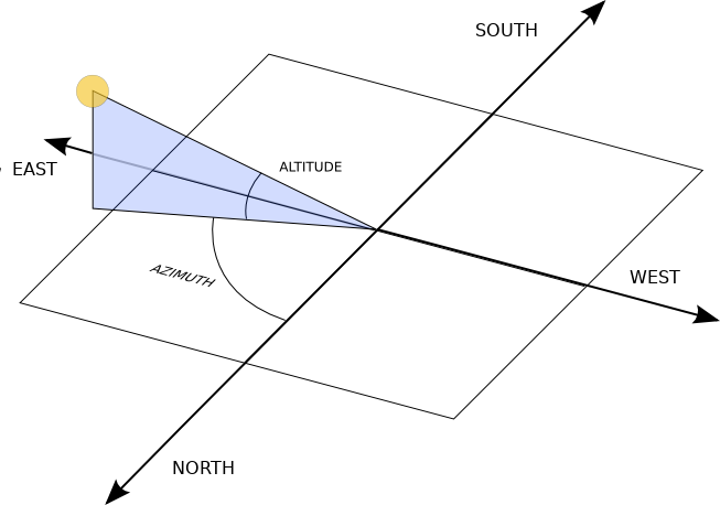
For the longest time I have wanted to explore the Pysolar package in python. It is a pretty great package that generates the azimuth and altitude of the sun based on a location and date/time (At its core, it does more as well). The image from the webpage explains it the best:
azi
Source: (https://pysolar.readthedocs.io/en/latest/)

It is a really great package, and doesnt need many inputs to get going. You can do alot more with it than just azimuth and latitude, but I will look at that later. I am goign to use four packages and python 3 (Pysolar no longer supports 2). The packages are:

In [66]:
import pysolar as ps
import datetime # to generate datetime objects
import pytz # generate a timezone object
import matplotlib.pyplot as plt # performing plots

The pysolar is pretty straight forward, and I will use mostly the altitude and azimuth functions. The functions which return the altitude of the sun, and the azumith with respect to north take three paramters:

  • Latitude;
  • Longitude; and
  • Date and Time

The latitude and longitude are pretty easy to generate using google maps (thought I am sure that there is some cleaver python package that can generate those from your address).My current location is in Chestermere Alberta, a small city located to the east of Calgary. The coordinates of my local dog park are taken from google maps:

In [67]:
lat_me = 51.0574094,
long_me = -113.8238714

The date and time can be a bit tricky I have found. This is because you need to specify the correct timezone for your location. I am assuming this is because the math is based from a UTC time, and then is corrected for the time offset. I did something similar to this once in a renewable energy class. Iam pretty sure we did the same calculation as pysolar does here!!

We can create a date and time by using the datetime library and inputting the following:

In [68]:
mst = pytz.timezone('Canada/Mountain')
date = datetime.datetime(2019, 7, 15,12,0,0,0,mst)

Note that we have specified the timezone using the pytz library. This is a datetime object for July 15, 2019 at 12:00 MST.

In [69]:
print(ps.solar.get_altitude(lat_me, long_me, date))
print(ps.solar.get_azimuth(lat_me, long_me, date))
[60.38700076]
[176.58495117]

Note the strange warning for leap seconds for after 2019!

Now we can start doing some interesting things. One item I have wanted to create for a long time is analemma. This is when you take the position of the sun at everyday, at the same time over a year or so. Taken from the wiki page here is a great example:

Analemma

We can generate an example of one of theses, by looping through all the months of the year at a specific time:

In [70]:
azi = []
alti = []
ana_date = datetime.datetime(2019,1,1,9,0,0,0,mst) # First date of the year

for month in range(0,364):
    ana_date = ana_date + datetime.timedelta(days=1) # increment by a single day
    altitude = ps.solar.get_altitude(lat_me, long_me, ana_date)
    azimuth = ps.solar.get_azimuth(lat_me, long_me, ana_date)
    azi.append(azimuth)
    alti.append(altitude)
    
plt.scatter(azi, alti)
Out[70]:
<matplotlib.collections.PathCollection at 0x7f4aa5cfbba8>
In [71]:
azi = []
alti = []
ana_date = datetime.datetime(2019,1,1,12,0,0,0,mst) # First date of the year

for day in range(0,364):
    ana_date = ana_date + datetime.timedelta(days=1) # increment by a single day
    altitude = ps.solar.get_altitude(lat_me, long_me, ana_date)
    azimuth = ps.solar.get_azimuth(lat_me, long_me, ana_date)
    azi.append(azimuth)
    alti.append(altitude)
    
plt.scatter(azi, alti)
Out[71]:
<matplotlib.collections.PathCollection at 0x7f4aa5a13eb8>

We can look at the curve of the sun over a day, by selecting a day and iterating over the hours

In [72]:
azi = []
alti = []

for hour in range(24):
    date_time = datetime.datetime(2019, 9, 15,hour,0,0,0,mst)
    altitude = ps.solar.get_altitude(lat_me, long_me, date_time)
    azimuth = ps.solar.get_azimuth(lat_me, long_me, date_time)
    azi.append(azimuth)
    alti.append(altitude)
In [73]:
plt.scatter(azi, alti)
Out[73]:
<matplotlib.collections.PathCollection at 0x7f4aa5ac35c0>

Based on this, on september 15 the sun peak at about 42 degrees. Intuitively I though this would be higher.Notice that there are negative numbers for the altitude. This makes sense as the sun is behind the earth during the nighttime hours!!!

To fix this, we can get a bit more specific with the plotting:

In [74]:
fig, ax = plt.subplots()
ax.scatter(azi, alti)
ax.set_ylim([0,45])
Out[74]:
(0, 45)

Finally we can combine the two items to create an analemma for every hour throughout the year. I would love to see someone do this with photography, if it is possible. Potentially an panaramic image that spans from east to west, every hour on the hour for every day.

In [75]:
azi = []
alti = []

for hour in range (0,23,1):
    ana_date = datetime.datetime(2019,1,1,hour,0,0,0,mst) # First date of the year, at hour 0
    for day in range(0,365):
        ana_date = ana_date + datetime.timedelta(days=1) # increment by a single day
        altitude = ps.solar.get_altitude(lat_me, long_me,ana_date)
        azimuth = ps.solar.get_azimuth(lat_me, long_me, ana_date)
        azi.append(azimuth)
        alti.append(altitude)
In [76]:
fig, ax = plt.subplots(figsize = (12,6))
ax.scatter(azi, alti)
ax.set_ylim([0,70])
Out[76]:
(0, 70)

Thats it for now on the begining use of this great library. Next time I look into it, I want to get the solar radiation values for a specific location. I have looked into the docs and there are some really interesting functions for radiation values.